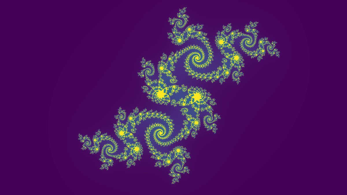
Visualize fractals of the Julia type in the Julia programming language. Under development.
Source can be found on GitLab.
Description of the Julia language
Implementation of the Julia fractal in the Julia programming language. The Julia language was chosen for this project mostly to check it out; the goal of the language is, among other things, to be as fast as C or Fortran, as expressive as Python, as good for statistics as R, to allow massively parallelization on the CPU and offloading work to GPUs as well as easy interfacing to beforementioned programming languages. I imagine it will be quite beneficial to the HPC community. This project is also a playground for experimenting with parallelization, optimizations, data visualization and running stuff on the GPU (when I get a new computer).
The Julia fractal
The resulting image with width \(M\) and height \(N\) of the fractal is created by plotting an image matrix \(I(M,N)\). Each pixel in the image, corresponding to an entry in the matrix, represents a point \(z\) in the complex plane.
Basically we need two functions julia_iter for calculating the function value of a single point and compute_fractal for calculating the entire image matrix.
function julia_iter(z::ComplexF64, c::ComplexF64, max_iter::Int64, ϵ::Float64)::Int

    """ Given a point z in the complex plane, calculate the function value

    :param z: point in the complex plane
    :param c: complex seed of the fractal
    :param max_iter: maximum number of iterations
    :param ϵ: escape criterion, set to R > 0 such that R**2 - R >= sqrt(Re(c)^2 + Im(c)^2)

    :return: function value, corresponding to the color in the fractal as a range between 0 and 255 (maximum)

    """

    for i in 1:max_iter

        z = z^2 + c

        if abs2(z) > ϵ

            return i

        end

    end

    return 255 # corresponding to maximum possible color value

end
Resulting fractal
Video with increasing max iterations
The maximum number of iterations defines how many iterations are “enough” before defaulting to the maximum of 255. Usual values are 80 to 200. A smaller number gives a more “smooth” looking fractal with less details, while a higher number gives the “true” fractal.
Video with zoom
One of the features of fractals, which also makes them interesting and mesmerezing to look at, is the property of repeated patterns when zooming in on a particular area of a fractal. Below is an example with a carefully selected origin \((x,y) = (-0.393772, 0.00717)\). This one takes a lot of time (and memory) to render as it is in 60 fps for a smooth video.
The video is currently not working for some reason. It’s probably better to host it myself when this site is moved to a raspberry pi (and I get a static IP).
Video with rotation of input seed
It is also nice to see the evolution when changing the input seed. Here it is changed as \(e^{i\cdot x}\) on the interval \([0:2\pi]\).
How to run
Locally
- Clone the repo
- Make sure you have Julia installed. Only tested with version 1.6.3 but should work with 1.5 as well.
- Run
using Pkg; activatefrom the Julie REPL (invoked with julia from the shell). This installs all dependencies (sort of likepip install -r requirements.txtfor Python projects) - Run the notebook either with
jupyter notebookfrom the shell orIJulia; notebook()from the Julia REPL - Read the setup section of the notebook
With Binder
You can also run the notebook with Binder here. Binder is a free service to run Jupyter/IJulia notebooks on the cloud that also takes care of all the project dependencies and so on. It might take some time to launch and also the limit is 2 GB memory and only 1 CPU core, so the multithreading parts are of no benefit. The future GPU code also probably won’t run.
